This story on climate change science originally appeared in science magazine EOS and is part of Covering Climate Now, a global journalism collaboration strengthening coverage of the climate story.
Has this happened to you? You are presenting the latest research about climate change to a general audience, maybe at the town library, to a local journalist, or even in an introductory science class. After presenting the solid science about greenhouse gases, how they work, and how we are changing them, you conclude with “and this is what the models predict about our climate future…”
At that point, your audience may feel they are being asked to make a leap of faith. Having no idea how the models work or what they contain and leave out, this final and crucial step becomes to them a “trust me” moment. Trust me moments can be easy to deny.
As questions are answered and models evolve, they should not only reproduce past measurements, but they should also begin to produce similar projections into the future.
This problem has not been made easier by a recent expansion in the number of models and the range of predictions presented in the literature. One recent study making this point is that of Hausfather et al., which presents the “hot model” problem: the fact that some of the newer models in the Coupled Model Intercomparison Project Phase 6 (CMIP6) model comparison yield predictions of global temperatures that are above the range presented in the Intergovernmental Panel on Climate Change’s (IPCC) Sixth Assessment Report. The authors present a number of reasons for, and solutions to, the hot model problem.
Models are crucial in advancing any field of science. They represent a state-of-the-art summary of what the community understands about its subject. Differences among models highlight unknowns on which new research can be focused.
But Hausfather and colleagues make another point: As questions are answered and models evolve, they should also converge. That is, they should not only reproduce past measurements, but they should also begin to produce similar projections into the future. When that does not happen, it can make trust me moments even less convincing.
Are there simpler ways to make the major points about climate change, especially to general audiences, without relying on complex models?
We think there are.
Old Predictions That Still Hold True
In a recent article in Eos, Andrei Lapenis retells the story of Mikhail Budyko’s 1972 predictions about global temperature and sea ice extent. Lapenis notes that those predictions have proven to be remarkably accurate. This is a good example of effective, long-term predictions of climate change that are based on simple physical mechanisms that are relatively easy to explain.
There are many other examples that go back more than a century. These simpler formulations don’t attempt to capture the spatial or temporal detail of the full models, but their success at predicting the overall influence of rising carbon dioxide (CO2) on global temperatures makes them a still-relevant, albeit mostly overlooked, resource in climate communication and even climate prediction.
Related articles: The Link Between Climate Change, the Environment, and our Health | Our Emissions Are Aggravating Almost 60% of All Infectious Diseases
One way to make use of this historical record is to present the relative consistency over time in estimates of equilibrium carbon sensitivity (ECS), the predicted change in mean global temperature expected from a doubling of atmospheric CO2. ECS can be presented in straightforward language, maybe even without the name and acronym, and is an understandable concept.
Estimates of ECS can be traced back for more than a century (Table 1), showing that the relationship between CO2 in the atmosphere and Earth’s radiation and heat balance, as an expression of a simple and straightforward physical process, has been understood for a very long time.
We can now measure that balance with precision [e.g., Loeb et al.], and measurements and modeling using improved technological expertise have all affirmed this scientific consistency.
Table 1. Selected Historical Estimates of Equilibrium Carbon Sensitivity (ECS)
| Date | Author | ECS (°C) | Notes |
|---|---|---|---|
| 1908 | Svante Arrhenius | 4 | In Worlds in the Making, Arrhenius also described a nonlinear relationship between CO2 and temperature. |
| 1938 | Guy Callendar | 2 | Predictions were based on infrared absorption by CO2, but in the absence of feedbacks involving water vapor. |
| 1956 | Gilbert Plass | 3.6 | A simple climate model was used to estimate ECS. Plass also accurately predicted changes by 2000 in both CO2 concentration and global temperature. |
| 1967 | Syukuro Manabe and Richard T. Wetherald | 2.3 | Predictions were derived from the first climate model to incorporate convection. |
| 1979 | U.S. National Research Council | 2–3.5 | The results were based on a summary of the state of research on climate change. The authors also concluded that they could not find any overlooked or underestimated physical effects that could alter that range. |
| 1990 to present | IPCC AR6 | 3 (2.5–4) | Numerous IPCC reports have generated estimates of ECS that have not changed significantly across the 30-year IPCC history. |
| 2022 | Hausfather et al. | 2.5–4 | ECS was derived by weighting models based on their historical accuracy when calculating multimodel averages. |
| 2022 | Aber and Ollinger | 2.8 | A simple equation derived from Arrhenius [1908] was applied to the Keeling curve and GISS temperature data set. |
Settled Science
Another approach for communicating with general audiences is to present an abbreviated history demonstrating that we have known the essentials of climate change for a very long time — that the basics are settled science.
The following list is a vastly oversimplified set of four milestones in the history of climate science that we have found to be effective. In a presentation setting, this four-step outline also provides a platform for a more detailed discussion if an audience wants to go there.
- ~1860: John Tyndall develops a method for measuring the absorbance of infrared radiation and demonstrates that CO2 is an effective absorber (acts as a greenhouse gas).
- 1908: Svante Arrhenius describes a nonlinear response to increased CO2 based on a year of excruciating hand calculations actually performed in 1896. His value for ECS is 4°C (Table 1), and the nonlinear response has been summarized in a simple one-parameter model.
- 1958: Charles Keeling establishes an observatory on Mauna Loa in Hawaii. He begins to construct the “Keeling curve” based on measurements of atmospheric CO2 concentration over time. It is amazing how few people in any audience will have seen this curve.
- Current: The GISS data set of global mean temperature from NASA’s Goddard Institute for Space Studies records the trajectory of change going back decades to centuries using both direct measurements and environmental proxies.
The last three of these steps can be combined graphically to show how well the simple relationship derived from Arrhenius’s projections, driven by CO2 data from the Keeling curve, predicts the modern trend in global average temperature (Figure 1). The average error in this prediction is only 0.081°C, or 8.1 hundredths of a degree.
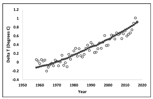
A surprise to us was that this relationship can be made even more precise by adding the El Niño index (November–January (NDJ) from the previous year) as a second predictor. The status of the El Niño–Southern Oscillation (ENSO) system has been known to affect global mean temperature as well as regional weather patterns. With this second term added, the average error in the prediction drops to just over 0.06°C, or 6 one hundredths of a degree.
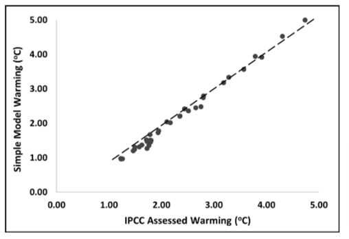
It is also possible to extend this simple analysis into the future using the same relationship and IPCC AR6 projections for CO2 and “assessed warming” (results from four scenarios combined; Figure 2).
Although CO2 is certainly not the only cause of increased warming, it provides a powerful index of the cumulative changes we are making to Earth’s climate system.
A presentation built around the consistency of equilibrium carbon sensitivity estimates does not deliver a complete understanding of the changes we are causing in the climate system, but the relatively simple, long-term historical perspective can be an effective way to tell the story.
In this regard, it is interesting that the “Summary for Policy Makers” from the most recent IPCC science report also includes a figure that captures both measured past and predicted future global temperature change as a function of cumulative CO2 emissions alone. Given that the fraction of emissions remaining in the atmosphere over time has been relatively constant, this is equivalent to the relationship with concentration presented here. That figure also presents the variation among the models in predicted future temperatures, which is much greater than the measurement errors in the GISS and Keeling data sets that underlie the relationship in Figure 1.
A presentation built around the consistency of ECS estimates and the four steps clearly does not deliver a complete understanding of the changes we are causing in the climate system, but the relatively simple, long-term historical perspective can be an effective way to tell the story of those changes.
Past Performance and Future Results
Projecting the simple model used in Figure 1 into the future (Figure 2) assumes that the same factors that have made CO2 alone such a good index to climate change to date will remain in place. But we know there are processes at work in the world that could break this relationship.
For example, some sources now see the electrification of the economic system, including transportation, production, and space heating and cooling, as part of the path to a zero-carbon economy. But there is one major economic sector in which energy production is not the dominant process for greenhouse gas emissions and carbon dioxide is not the major greenhouse gas. That sector is agriculture.
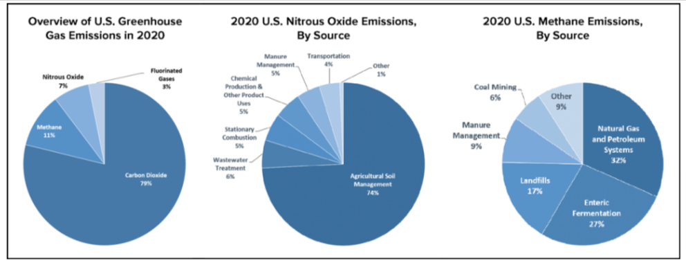
The US Department of Agriculture has estimated that agriculture currently accounts for about 10% of total US greenhouse gas emissions, with nitrous oxide (N2O) and methane (CH4) being major contributors to that total. According to the EPA (Figure 3), agriculture contributes 79% of N2O emissions in the United States, largely from the production and application of fertilizers (agricultural soil management) as well as from manure management, and 36% of CH4 emissions (enteric fermentation and manure management — one might add some of the landfill emissions to that total as well).
If we succeed in moving nonagricultural sectors of the economy toward a zero-carbon state, the relationship in Figures 1 and 2 will be broken. The rate of overall climate warming would be reduced significantly, but N2O and CH4 would begin to play a more dominant role in driving continued greenhouse gas warming of the planet, and we will then need more complex models than the one used for Figures 1 and 2. But just how complex?
In his recent book “Life Is Simple,” biologist Johnjoe McFadden traces the influence across the centuries of William of Occam (~1287–1347) and Occam’s razor as a concept in the development of our physical understanding of everything from the cosmos to the subatomic structure of matter. One simple statement of Occam’s razor is, Entities should not be multiplied without necessity.
This is a simple and powerful statement: Explain a set of measurements with as few parameters, or entities, as possible. But the definition of necessity can change when the goals of a model or presentation change. The simple model used in Figures 1 and 2 tells us nothing about tomorrow’s weather or the rate of sea level rise or the rate of glacial melt. But for as long as the relationship serves to capture the role of CO2 as an accurate index of changes in mean global temperature, it can serve the goal of making plain to general audiences that there are solid, undeniable scientific reasons why climate change is happening.
Getting the Message Across
If we move toward an electrified economy and toward zero-carbon sources of electricity, the simple relationship derived from Arrhenius’s calculations will no longer serve that function. But when and if it does fail, it will still provide a useful platform for explaining what has happened and why. Perhaps there will be another, slightly more complex model for predicting and explaining climate change that involves three gases.
No matter how our climate future evolves, simpler and more accessible presentations of climate change science will always rely on and begin with our current understanding of the climate system. Complex, detailed models will be central to predicting our climate future (Figure 2 here would not be possible without them), but we will be more effective communicators if we can discern how best to simplify that complexity when presenting the essentials of climate science to general audiences.
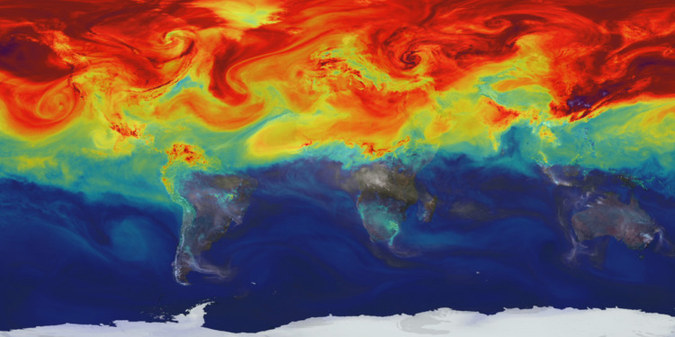
Editor’s Note: The opinions expressed here by the authors are their own, not those of Impakter.com — In the Featured Photo: A NASA supercomputer model provides a new portrait of a greenhouse gas. Featured Photo Credit: William Putman/NASA Goddard Space Flight Center.


